RH Saga Chapter 5.2: Lambda-ring operations

Given two L-functions $L_1$ and $L_2$, we can form their direct sum $L_1 \oplus L_2$, as well as their tensor product $L_1 \otimes L_2$. These two fundamental operations of addition and multiplication make the set $\mathbb{L}$ of all L-functions into a ring.

Given a single L-function $L$, we can, for any positive integer $k$, form it's $k$'th symmetric power L-function $Sym^k \ L$. This sequence of unary operations $Sym ^k$ makes $\mathbb{L}$ into a lambda-ring.

In addition to the symmetric power operations, there are other sequences of unary operations, notably the exterior power operations $Ext ^k$, the Adams operations $\psi ^k$, and the gamma operations $\gamma ^k$. Importantly, any one of these four sequences determines all the others, in the sense that there is a formula which expresses for example $Sym ^3$ in terms of $Ext ^1$, $Ext ^2$, $Ext ^3$, and each such formula is universal, i.e. the same for every lambda-ring. For this specific example, we have

\[ Sym ^3 = Ext ^1 \otimes Ext ^1 \otimes Ext ^1 \ominus 2 \cdot Ext ^1 \otimes Ext ^2 \oplus Ext ^3 \]

In this relation, I have also used the minus operation $\ominus$, which is defined in terms of addition as you would expect.

The purpose of this post is to explain what all these operations are, whereever possible in elementary terms, and to introduce some of the mysteries surrounding them.

Motivating examples

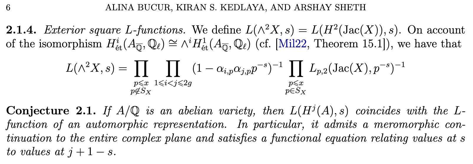
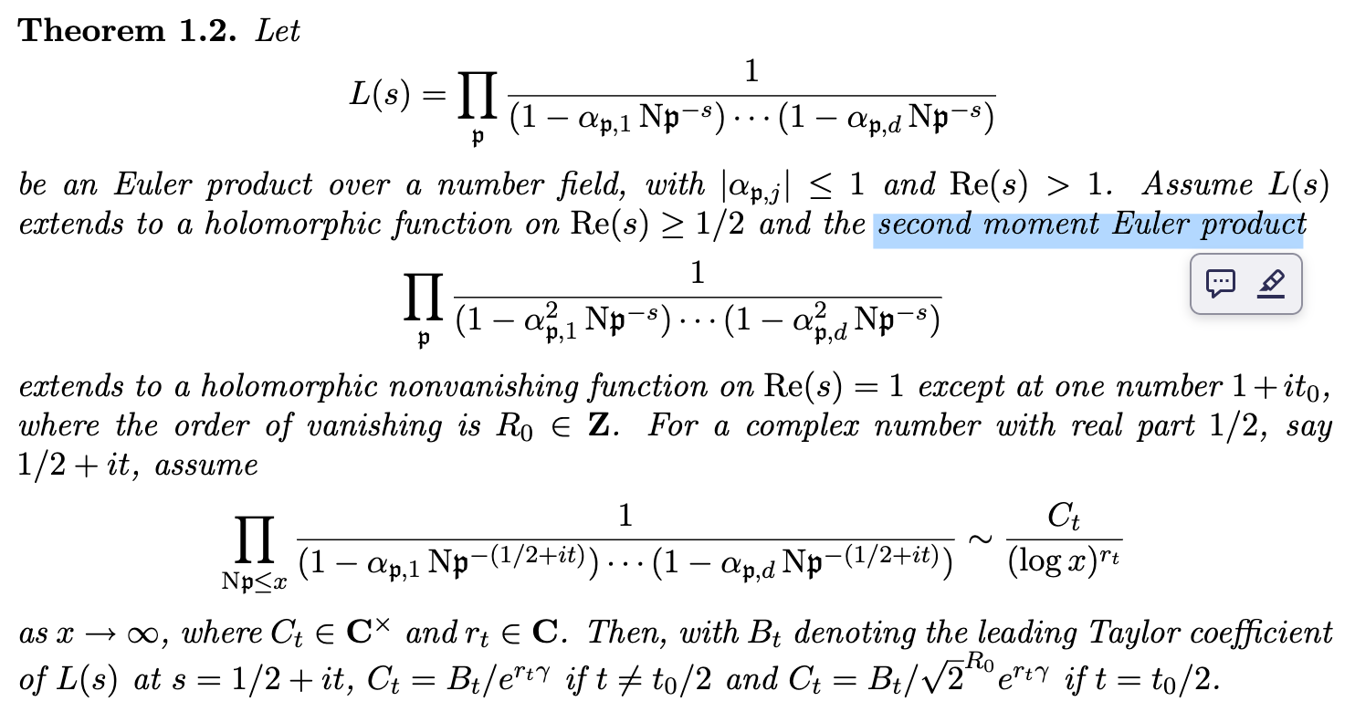
If you read the modern L-function literature, you will find these operations everywhere, although sometimes under different names. A basic example is that the L-function $L_K$ from the RH Saga videos (associated to the Gaussian integers) decomposes as a direct sum of the Riemann zeta function and the Dirichlet L-function we called $L_A$. You may recall from Chapter 4 that in the general theorem about zero-free regions for an L-function, Iwaniec and Kowalski had to assume the existence and some properties of the tensor product of $L$ with itself, as well as the tensor product of $L$ with its complex conjugate. You may also recall the short talk by Khare on the work of Newton and Thorne, where the symmetric powers played a central role. For two more examples, here is a screenshot from the recent preprint of Bucur, Kedlaya and Sheth, where they refer to the exterior square L-function $Ext^2$ (in their notation $\wedge ^2$), and another screenshot from an important paper of Conrad, where he uses $\psi ^2$, but under the name second moment Euler product.

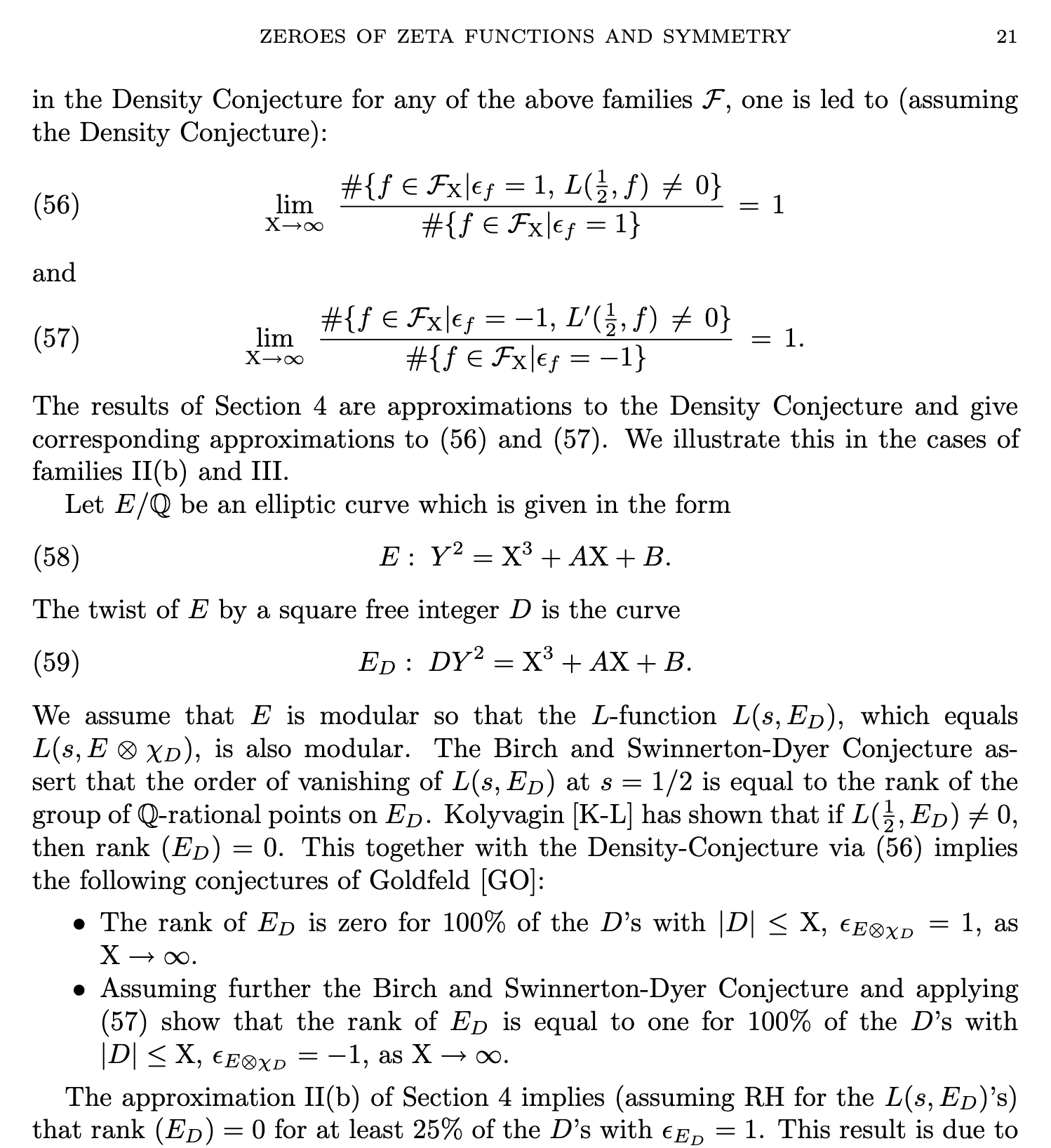
Sometimes we use the word twist for the tensor product of an L-function with a Dirichlet L-function, as for example in the screenshot below, from the Katz-Sarnak paper we talked about in Chapter 5.1.

Hopefully this small list of representative examples serves to illustrate the pervasive role that lambda-ring operations play throughout the theory of L-functions.

Analogous settings

You may in fact be familiar with operations like the above, without necessarily having used lambda-ring language. I'll describe three settings which can be helpful for understanding the somewhat more complicated L-function theory.

Lie groups and particle physics

If you have studied physics, you may be familiar with representations of Lie groups and the need to decompose tensor products of representations with the help of Clebsch-Gordan coefficients. Take $SU(3)$ as an example. For each pair $(p, q)$ of non-negative integers, there is an irreducible representation called $D(p, q)$, of dimension $\frac{1}{2}(p+1)(q+1)(p+q+2)$. The physical meaning of these numbers is that $p$ is the number of quarks, and $q$ the number of anti-quarks. A central problem is to understand what happens when you take the tensor product of two representations. As an example (taken from Wikipedia), you can take the tensor product of $D(1, 1)$ with itself, and this decomposes as the direct sum of six summands, like this:

Such decompositions have physical significance that I personally don't understand, but I can quote Sidney Coleman (page 9, where the above corresponds to Example 1): "This is a familiar (and useful) result. It tells us the number of independent amplitudes for the scattering of two octets into two octets (eight, if time reversal imposes no further restrictions), the number of independent Yukawa couplings for antibaryon-baryon-pseudoscalar meson (two), the number of amplitudes for the decay of a $\frac{3}{2} ^{+}$ resonance into baryon and pseudoscalar meson (one), etc."

Finite groups

Perhaps you are familiar with the character table of a finite group. Here's the character table for the symmetric group $S_3$ (the smallest non-abelian group), copied from some nice lecture notes of Vincent Bouchard.

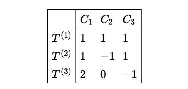
Think of the group as the symmetry group of an equilateral triangle. There are six elements naturally partitioned into three conjugacy classes: One identity, three flips, and two nontrivial rotations. The top row lists the respective conjugacy classes, labelled $C_1, C_2, C_3$. The rows correspond to the three irreducible representations of $S_3$, i.e. the trivial representation (of dimension 1, and I'll write $V_1$ instead of $T ^{(1)}$), the sign representation $V_2$ (of dimension 1), and the two-dimensional representation $V_3$. The character table lists the trace of a group element in the class $C_j$ on the representation $V_i$.

Using this table, it is very easy to compute direct sum and tensor products, as you can simply add or multiply two rows, element-by-element! For example, $V_3 \otimes V_3$ gives the row vector $(4, 0, 1)$, and the only way to write this vector as a linear combination of the three original ones is

\[ V_3 \otimes V_3 = V_1 \oplus V_2 \oplus V_3 \]

Symmetric polynomials

If you've solved math olympiad problems with symmetric polynomials, you will recall that there are different "bases" for them. For example, in two variables $x, y$ all symmetric polynomials can be expressed either in terms of the elementary polynomials $e_1 = x+y$ and $e_2 = xy$, OR in terms of the power sum polynomials $p_1 = x+y$ and $p_2 = x ^2+y ^2$. There is also another base, called the complete homogeneous symmetric functions, which sums up all possible monomials of a given degree. Using three variables as an illustration, the general pattern should become quite clear:

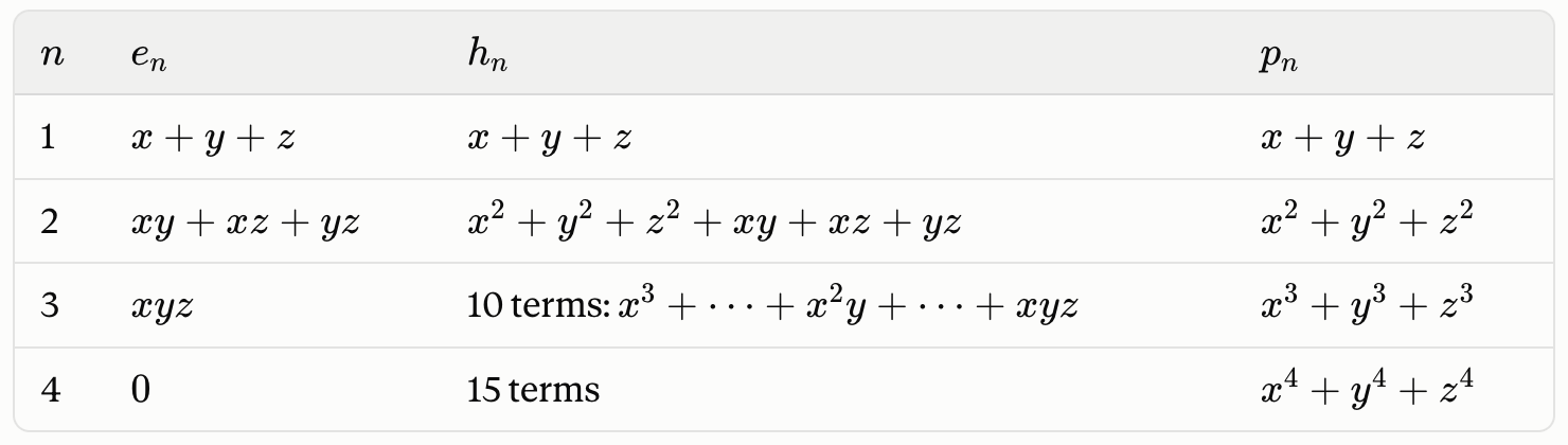
These three columns correspond in a precise way to the exterior power operations, the symmetric power operations, and the Adams operations (and there is fourth column for the gamma operations, omitted here).

The formalism of bases for symmetric polynomials is one way to understand the relation between the different sequences of unary operations. For example, you can see that the symmetric cube in the table (the one with 10 terms) can be expressed as

and this tells you precisely how to compute $Sym ^3$ in terms of $Ext ^1$, $Ext ^2$ and $Ext ^3$.

Operations on L-functions

In RH Saga Episode 5, definitions were given for direct sum, tensor product, and symmetric powers, and the other unary operations are defined similarly, following the patterns of the symmetric polynomial relations of the previous paragraph.

In general, these operations are performed Euler factor by Euler factor. Let us spell out these definitions again, for future reference.

Recall the fact that given an L-function, the Euler factor at a prime $p$ is of the form $\frac{1}{F_p(T)}$, where $F_p$ is a polynomial and $T$ is shorthand for $p^{-s}$. Here is a representative example from the LMFDB for the L-function of degree 4 associated to the first (by conductor) genus 2 curve:

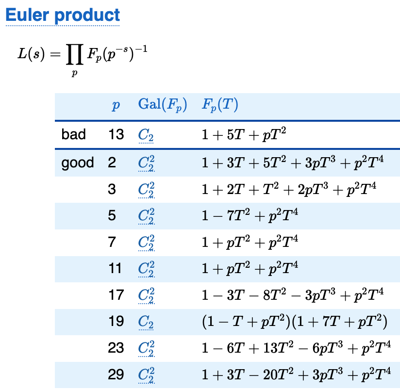
The conductor of this curve is $169$, so the only bad prime is $p=13$, and the table illustrates the general principle that all these "local polynomials" have the same degree (in this case $4$) except at the bad prime, where the degree is lower (in this case $2$).

The local polynomial factors over the complex numbers into linear factors of the form $(1-\alpha T)$, and the operations are defined in terms of these "reciprocal roots" $\alpha$. As an example, take $F_5(T) = 1-7T ^2 + 25 T ^4$ from the table above. A quick way to get the four reciprocal roots is to ask Wolfram Alpha for the roots of the reverse polynomial, like this.

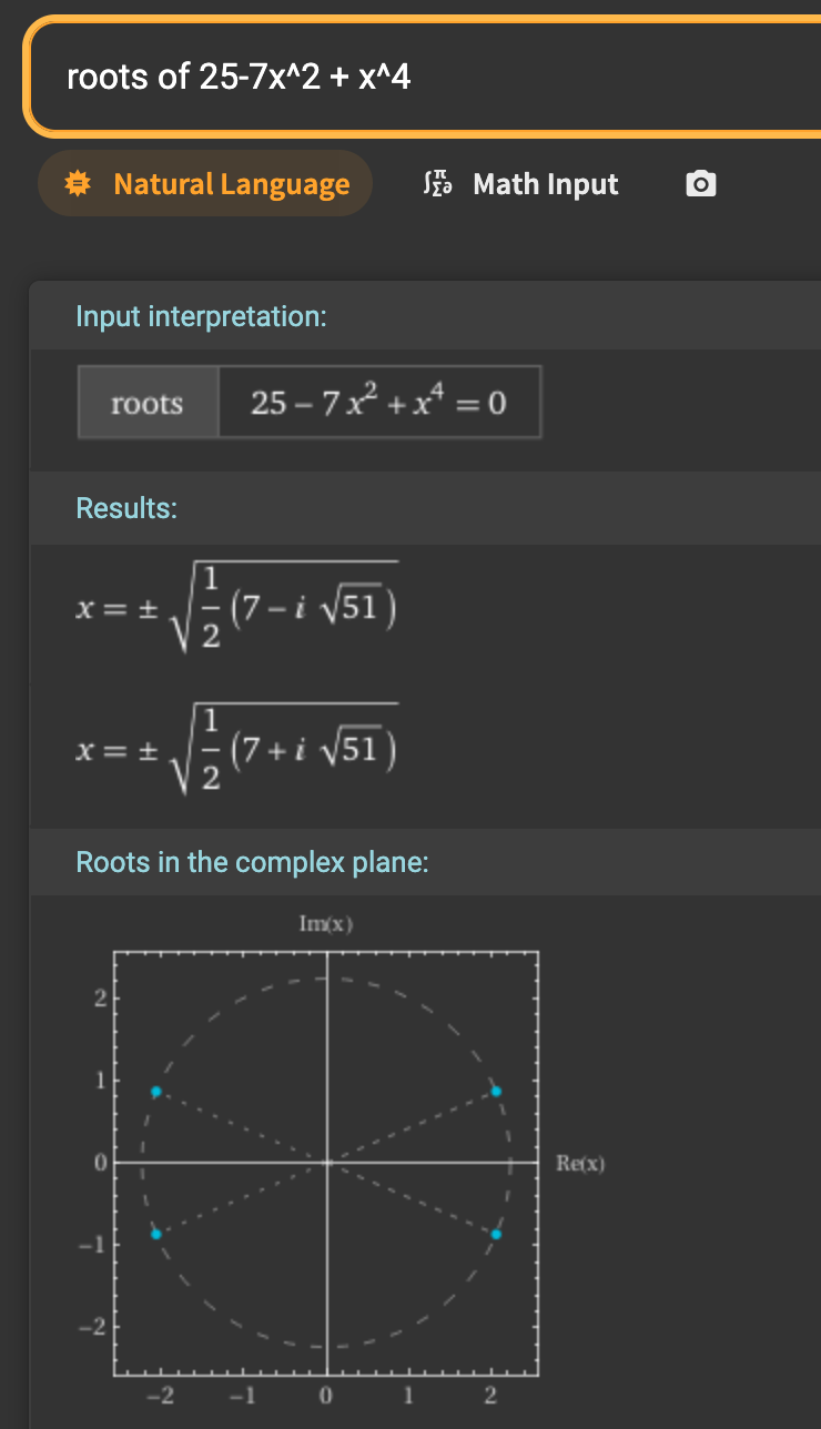
As indicated in the image, these numbers lie on a circle of radius exactly $\sqrt{5}$. That this is so is an instance of the local Riemann hypothesis, part of the Weil conjectures.

Addition and multiplication

Fix a prime $p$, and consider two L-functions whose local polynomial at $p$ is determined by the reciprocal roots $\{ \alpha_1, \alpha_2, \ldots , \alpha_m \}$ and $\{ \beta_1, \beta_2, \ldots , \beta_n \}$. These two sets (strictly speaking multisets, since repetition is allowed) form a very convenient representation of the local Euler factor, for the purpose of defining operations. We call such a multiset the Satake parameters of the L-function at the prime $p$.

The direct sum of two L-functions is now defined by taking, for each prime $p$, the disjoint union of the Satake parameters.

The naive tensor product of two L-functions is defined by taking, for each prime $p$, the multiset of products of the form $\alpha_i \beta_j$.

The tensor product of two L-functions is defined by taking the naive tensor product followed by a certain perturbation, i.e. a modification of a finite number of Euler factors. The Euler factors to modify correspond to a subset of the primes which were bad for at least one of the original L-functions.

Unary operations

Given one L-function and a prime $p$, let $ A = \{ \alpha_1, \ldots, \alpha_m \}$ be the list of Satake parameters. We can now define each unary operation by specifying what it does to this multiset.

• The Adams operation $\psi^k$ replaces each $\alpha$ by $\alpha ^k$.
• The symmetric power operation $Sym^k$ replaces the multiset $A$ by the multiset of all degree $k$ monomials formed from the $\alpha_i$. In the table of symmetric polynomials above, you see the sum of these monomials in the column for $h_n$.
• The exterior power operation $Ext ^k$ is defined by the subset of monomials which are products over distinct indices $i$. What this means should become clear if you again look at the table above, displaying the sum of these monomials in the column for $e_n$.

Important note: Each of the above operations should be called the naive Adams operation, the naive symmetric power, etc. The true operations require post-composition with a perturbation, as for the tensor product.

Note also that with the information I have given you here, you can verify any relation you wish in the context of a general lambda-ring! Take for example the formula for $Sym^3$ given in the introduction. Let's check it. Using a set of two elements $a, b$ as our multiset, you will easily find:

• $Sym ^3 = \{ a ^3, a ^2 b, a b ^2 , b ^3\}$
• $(Ext ^1) ^{\otimes 3} = \{ a, b \} \otimes \{ a, b \} \otimes \{ a, b \} = \{ a ^3, 3 \cdot a ^2 b, 3 \cdot a b ^2 , b ^3\}$ (the $3$ simply means three copies of that element).
• $ Ext ^1 \otimes Ext ^2 = \{ a, b \} \otimes \{ ab \} = \{ a ^2 b, a b ^2 \}$
• $Ext ^3 = \emptyset$ (the empty multiset).

Now check that the first multiset is obtained from the second by "subtracting" twice the third and "adding" the last one. You can also redo the same computation for three elements (or any larger number) to convince yourself that the relation is independent of the number of elements, and not, for instance, an artifact of the incidental empty multiset we had.

The mystery of the bad primes

For many years, I have tried consulting the literature and asking experts about how one can understand the nature of the required corrective perturbation for all of the above operations, at bad primes. The brief answer is that this is understood in principle, it's related to the local Langlands correspondence and Weil-Deligne representations, but it is genuinely difficult to make things explicit/elementary. In the simplest of all cases, for two of our Dirichlet L-functions $L_D$, the tensor product can be made explicit, as we saw in the tables back in Chapter 2.

It has been a small dream of mine to reformulate the very abstract technicalities from the local Langlands story into some kind of elementary explanation for how to compute tensor product and all of the unary operations. I am planning to share a series of separate posts on this problem, in the hope that I will understand more by doing so, and that someone else may be encouraged to explain things to me or to work out this idea beyond what I have been able to do.

I should mention also that in many practical situations, the mysterious Euler factors are determined not by understanding what happens locally (i.e. at the prime $p$), but by applying the global compatibility requirement called the functional equation, which constrains the product of all the Euler factors. To give an example of such a situation, here is a screenshot of a summary from a workshop on hypergeometric motives. Note the formulation in point 5 on the bad Euler factors; I believe this setting is one where the complexity of the local Langlands story is simply far too high even for the leading experts to attempt a direct, theoretical calculation.