RH Saga Chapter 5.1: Families of L-functions

At the phenomenological level this is perhaps the most striking discovery about zeta since Riemann.

Let's keep going in our quest for clues for a possible theory of the field with one element! Last time, we emphasized the importance of viewing L-functions not as isolated objects but as a part of a greater whole. Today, I want to dive into specifics around families of L-functions. A family is simply a sequence $L_1$, $L_2$, $L_3$, of L-functions. Sometimes the family is not presented in the form of a sequence, but rather as "the set of all L-functions with properties so-and-so". But in this case, we can still make the family into a sequence, by imposing an ordering by the size of some invariant, like the degree, or the conductor, or by a more refined invariant (applicable to any family) called the analytic conductor. This invariant will be discussed and defined properly in Chapter 6, but you can think of it for now as the usual conductor multiplied by some extra stuff related to the Gamma factor of the L-function.

For virtually every mathematical concept, moving from the study of isolated objects to sequences of objects will open up new perspectives and routes to insights also about the original objects. You might not have cared deeply about the number $144$ until you learnt that it is the largest Fibonacci number which is a perfect power of another number. But this fascinating fact about the single number $144$ (proved by Bugeaud, Mignotte and Siksek) cannot even be stated unless you have in your language the ability to think about the Fibonacci sequence and sequences of squares, cubes, and so on. If you care about a single topological space $X$, you will need to think about the sequence $X_1$, $X_2$, $X_3$, ..., forming its Postnikov tower, and similarly for other mathematical concepts. So it should not come as a surprise that sequences of L-functions are important!

For the material in this chapter, a nice survey is Conrey: L-functions and random matrices, from 2000. Another very important paper is the classical 1999 paper of Katz and Sarnak called Zeros of zeta functions and symmetry, from which the opening quote is taken, referring to Odlyzko's computations confirming the random matrix model (GUE) predictions.

A new aspect of the Rosetta Stone

There are many facets to the analogy between function fields and number fields, and we are now focussing on the statistics of zeros of L-functions in each of these worlds, together with geometric ideas well understood on the function field side, like monodromy and a spectral interpretation of the zeros. Below is a table taken from Katz and Sarnak, page 12, where you see a list of the main ideas. Point 4 is the Riemann Hypothesis. Point 5 concerns statistical patterns for the zeros of an individual L-function, and point 6 is related to zeros in a family of L-functions. Sometimes you will see these described as the "high zeros of an individual L-function" and the "low zeros of a family" (or "low-lying" zeros). Both of these are important and we will discuss them below.

Point 2 below relates to $\mathbb{F}_1$ in that known proofs of the functional equation (in the number field world) uses Poisson summation or automorphic theory, but some future $\mathbb{F} _1$-geometry might come with new proofs more in the style of function fields, involving some (yet unknown) notions similar to étale cohomology and the Riemann-Roch theorem. This will not be discussed today, but in future chapters.

Finally, point 3 asks whether the zeros of an L-function have some kind of spectral interpretation, meaning that they are (or are related to) the eigenvalues of some matrix or operator.

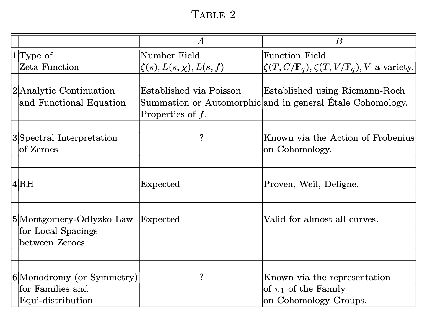
I'll try to explain a bit more about each of these points.

Statistics for an individual L-function

It turns out that as you study the nontrivial zeros of an L-function, arranged by increasing imaginary part and presumably all lying on the critical line, there seems to be a universal statistical pattern, valid for every single L-function, called the GUE random matrix model ("Grand Unitary Ensemble").

To get a first feeling for what this means, here is a picture of the first 60 zeros for the Dirichlet L-function with $D=5$.

In this picture, the zeros (marked as blue bands) are compared with the green bands underneath, depicting a different kind of distribution which one would expect to see if the L-function zeros appeared on the critical line "independently of each other", which in more precise mathematical language is expressed as the zeros appearing in a "Poisson process". As you can see, the actual zeros (in blue) tend to "repel" each other, refusing to huddle together in tight groups, although on rare occasions two of them might find the courage to sniff each other out.

I would like to say that the blue bands represents the imaginary parts of the zeros, but this is not literally true. Instead, they represent the "unfolded" zeros, meaning that the imaginary parts have been rescaled slightly so that instead of gradually becoming more dense as we move up the critical line, they keep coming with mean distance $1$. Algebraically, each imaginary part $\gamma$ of a zero has been replaced by the expression (called the "unfolding")

\[ \tilde{\gamma} = \frac{\gamma}{2 \pi} \log \frac{N \gamma}{2\pi e} \]

where $N=\vert D \vert$ is the conductor of the L-function.

One way to express the GUE idea more precisely is to look not just at the distance between consecutive zeros, but between all pairs of zeros, using a statistic called the "pair correlation". If we order the "spectrum" of an L-function by the positive imaginary parts $\gamma_1$, $\gamma_2$, $\gamma_3$, ..., then the pair correlation conjecture can be formulated as follows, and here I will simply screenshot a paragraph from Rubinstein: Computational methods and experiments in analytic number theory (page 44).

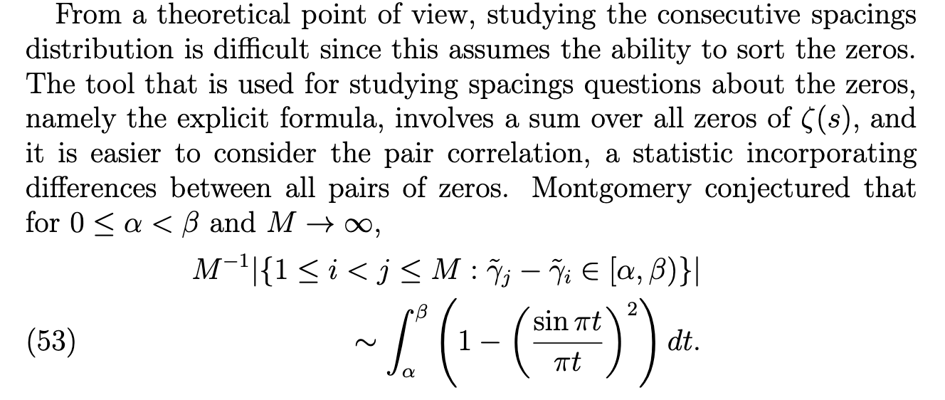
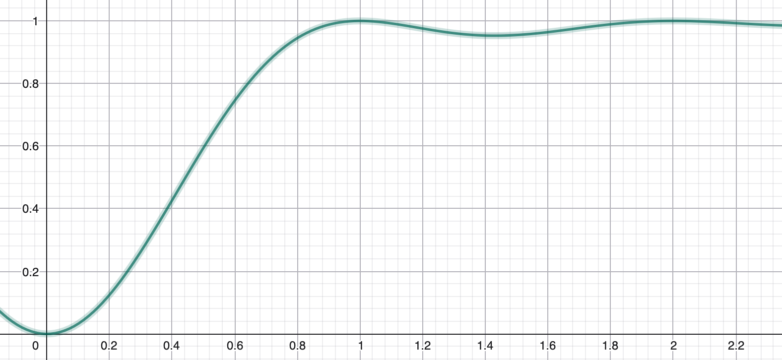
Parsing this statement, the idea is that if you look at the first $M$ zeros of zeta, take any interval $[ \alpha, \beta)$ (say from $0.4$ to $0.6$), and count how many pairs of your zeta zeros have a mutual distance in this interval, then a good estimate for that count is the integral of the function graphed below (over your chosen interval), multiplied by $M$. As $M$ grows larger, the estimate grows more accurate. You can eyeball the integral for our chosen interval from the graph to be around $0.12$ (use the midpoint method!), so among the first 1 000 zeta zeroes (and hence the almost 1 000 000 pairs!), you will find around 120 pairs of zeros (not necessarily neighbours!) with mutual distance within $0.5 \pm 0.1$. The fact that the graph takes very small values near zero (in fact it vanishes to order 2 there) tells you precisely that it is very rare for pairs to huddle together.

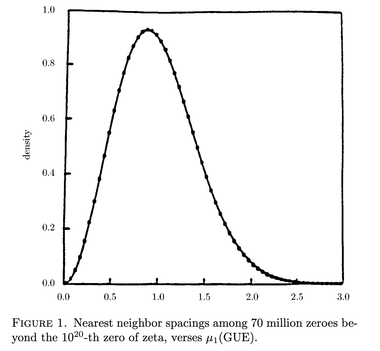
Historically, an important chapter of this story was the numerical work of Odlyzko in the 80s, in which he computed 70 million Riemann zeta zeroes situated very high up on the critical line, around height $10^{20}$, since with this data he could verify numerically the prediction of the pair correlation conjecture. The graph below show the GUE-predicted distribution not for all pairs (as in the previous graphs), but for consecutive pairs only, and the dots represent Odlyzko's experimental results. You can see from the graph that when the zeros are rescaled to have mean consecutive distance 1, it is very rare for such a distance to ever exceed 2.5, but anything below that number is reasonably common.

Other L-functions have also been investigated numerically, supporting the idea that every L-function satisfies exactly the same "GUE" statistical law for consecutive spacings of the zeros, with the fit being more accurate if you go high up on the line, and if you sample many zeros. Here are two more graphs from Katz and Sarnak, for the L-function of the Ramanujan $\Delta$ function, and the L-function of an elliptic curve, where fewer zeros were sampled.

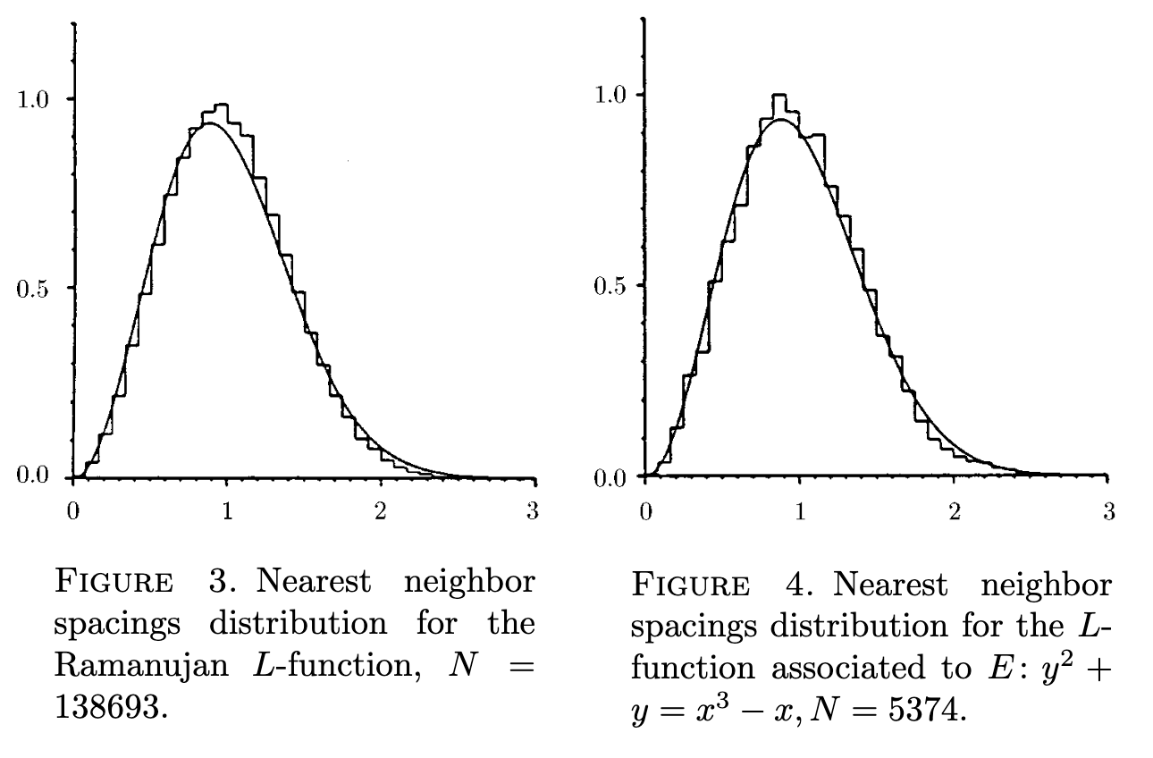
The paper by Rubinstein just mentioned is a very nice source for learning more, see in particular section 4, from page 42. The principle that the distances between zeros of any L-function behave in this way is called the "Montgomery-Odlyzko Law".

One interesting detail is that in order to achieve mean spacing 1, the precise form of the rescaling (or "unfolding", or "renormalization") depends on the degree and the conductor of the L-function. For Dirichlet (degree 1) L-functions of conductor $N$, the formula was given above. For elliptic curve L-functions (degree 2), one must use

These formulas are taken from Rubinstein, and reflect the general shape of the counting function for an L-function, which is

\[ N(T) = \frac{T}{2 \pi} \log \frac{N T^d}{(2 \pi e)^ d} + \textrm{error term} \]

where $N(T)$ on the left hand side is the number of zeros with imaginary part between $0$ and $T$, for an L-function of degree $d$, and where $N$ on the right hand side means the conductor.

How should one think of these statistical patterns? What number-theoretic consequences do they have? One way to think about it is that the Riemann Hypothesis governs where the zeros lie in the horizontal direction, while the GUE random matrix model is a refinement of GRH which governs where the zeros are located (in relation to each other) in the vertical direction. The Riemann hypothesis tells us that second Chebyshev function $\psi(x)$ (see Chapter 3) satisfies

\[ \psi(x) - x = O (\sqrt{x} \cdot \textrm{logarithmic factor} ) \]

and it is an open question (related to the "deep Riemann hypothesis") how small one can make this logarithmic factor. The pair correlation conjecture implies a sharpened form of this factor; see the 2022 paper of Goldston and Suriajaya for details. A side comment here is that there is another kind of hypothesis, saying that the imaginary parts of the zeros are linearly independent over $\mathbb{Q}$), which can also be used to prove sharpenings of the logarithmic factor. See the recent paper of Ng for an introduction to these ideas. Perhaps a very crude (and possibly misguided) intuition for these two mechanisms could be that even if RH is true (so that the square root is the correct power factor of the error term), there are two ways in which the zeros (i.e. frequencies of the wave functions) might still conspire towards a weak logarithmic factor, namely either by often clustering closely together, or by being integer multiples of each other (or more generally having $\mathbb{Q}$-linear relations).

There is a version of the Montgomery pair correlation conjecture which is actually a theorem (by Baluyot, Goldston, Suriajaya, and Turnage-Butterbaugh). Quite remarkably, a new proof appeared on arXiv very recently of the fact that at least 67.25 percent of the zeros of the Riemann zeta function are simple and on the critical line, based on this pair correlation theorem, and this new proof, by Lamzouri, is simpler than the proof by Claude that appeared a few weeks earlier. I am not really familiar with the details of these recent developments, but you can check out Lamzouri's paper and the papers of Baluyot et.al. on the arXiv.

Another interesting point is that the pair correlation conjecture (even for just the Riemann zeta function) has consequences in terms of bounds for class numbers of imaginary quadratic fields. See the introductory discussion in Conrey and Iwaniec, in their "lowest arXiv identifier digit sum world record" paper.

Everything said so far concerns the zeros of an individual L-function. We now turn to a different kind of random matrix model, predicting the behaviour of families of L-functions.

Statistics for a family of L-functions

For a family of L-functions, there are patterns in their low-lying zeroes which suggest an analogy with what's called the monodromy group in the function field world. This is interesting, since monodromy was a key ingredient in Deligne's proof of the Riemann Hypothesis for varieties over finite fields in 1973.

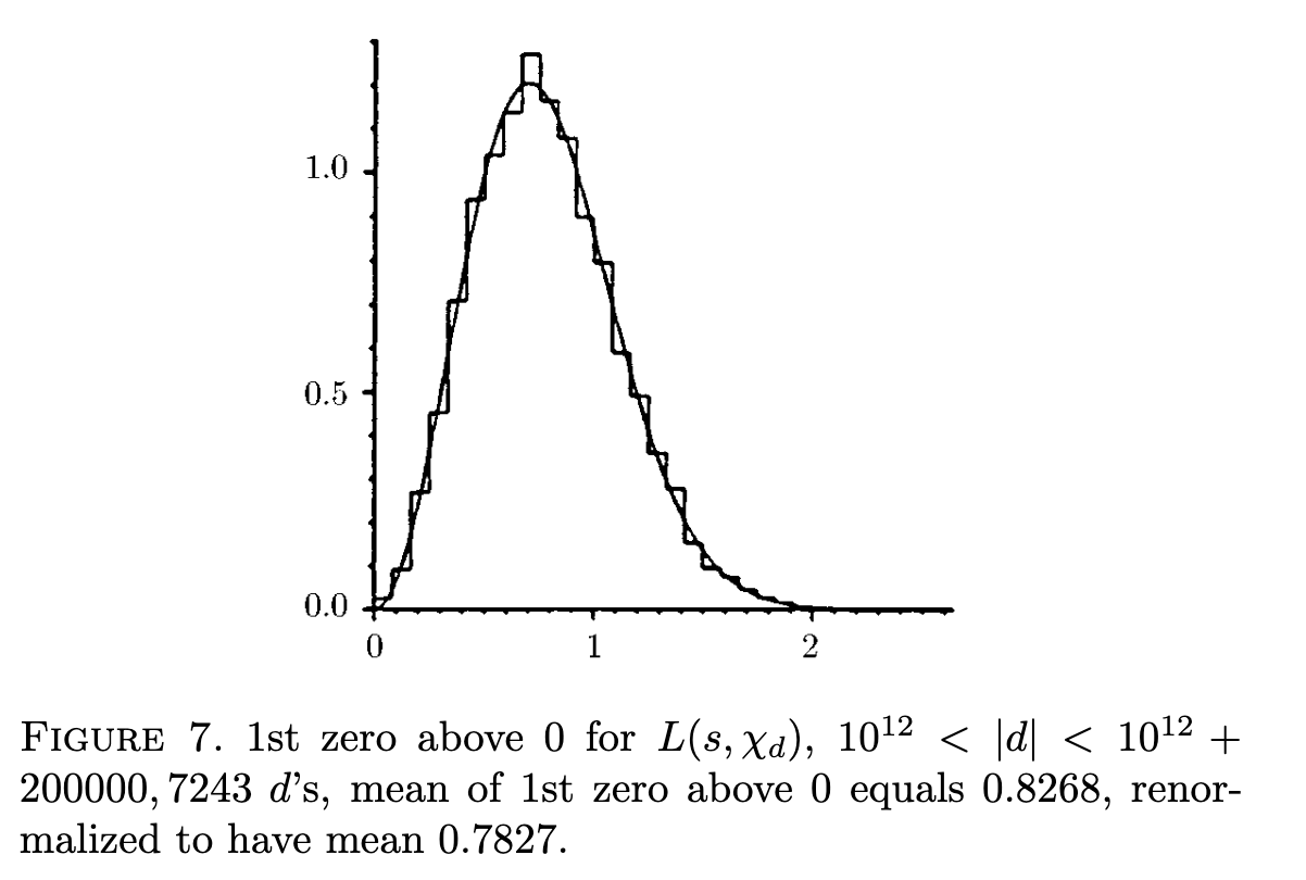
To give a first idea of what these patterns are, consider the family of quadratic Dirichlet L-functions we have seen many times. For each such L-function $L_D(s)$, we can take note of the lowest zero with strictly positive imaginary part. Plotting these zeroes (rescaled as earlier), we get a histogram like the one below, where a certain smooth graph has also been overlaid.

If you forget all about L-functions for a moment, and instead simply study eigenvalues of a random matrix, the smallest eigenvalue can be shown to obey a distribution that depends on which matrix group you sample the random matrix from. Here are some graphs, which illustrate these distributions for a unitary group $U(N)$, a symplectic group $USp(2N)$, and a special orthogonal group $SO(2N)$, and these graphs are obtained in the limit as $N \to \infty$.

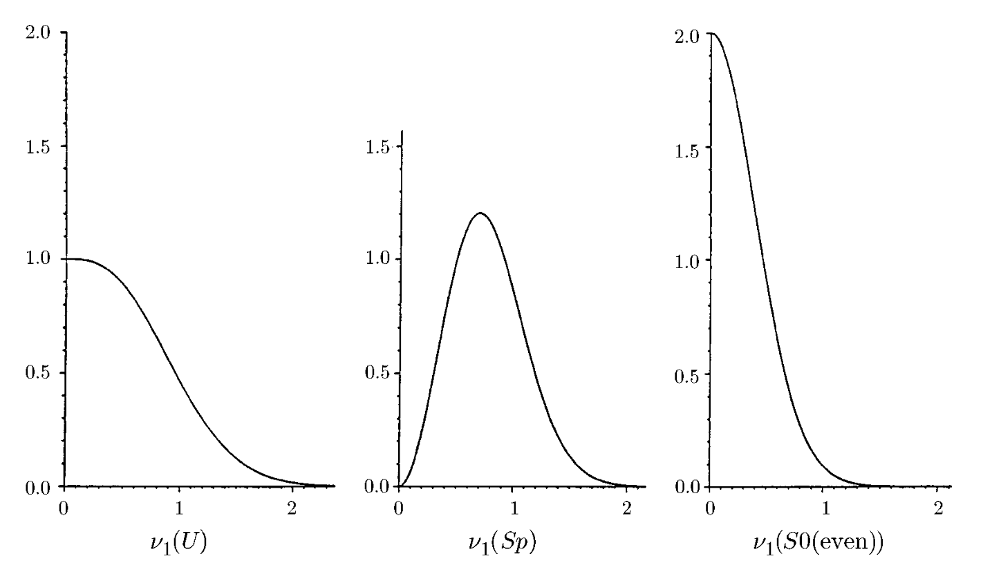
If you compare with the lowest-zero statistics for the Dirichlet L-functions in the preceding graph, you will see that the zeros of this L-function family behave as if they were sampled from the same distribution as the lowest eigenvalue of a large unitary symplectic matrix.

Of course, one has to be somewhat careful in interpreting what this "really means". Just like the prime numbers are not random objects, but can still be modelled by random variables for the purpose of making certain predictions, the list of lowest zeros are specific "deterministic" numbers, but in aggregate, they tend to follow a distribution which is the same as that of a certain random variable.

Let's consider a more advance example of a family of L-functions. We can take the L-function of the Ramanujan $\Delta$-function and twist it (i.e. take the tensor product) with a Dirichlet L-function $L_D$. By varying $D$, we get an interesting family, and the histogram below shows the first zero like before, for a certain range of Dirichlet characters with $D>0$.

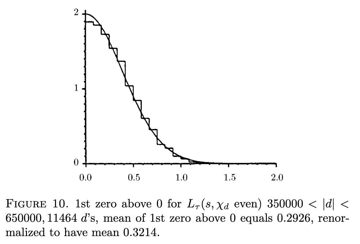
As you can see, this looks suspiciously like the lowest eigenvalue statistics for the special orthogonal group above!!

These two examples should be enough to convey the gist of the strange connection between the lowest zero in a family of L-functions and the lowest eigenvalue of a random matrix of a certain type.

Now, similar statistical patterns hold not just for the first zero, but also for the second-lowest and more generally for subsequent "low-lying zeros" of L-functions in a family. Extensive numerical evidence suggests that the there are essentially only three kinds of statistical behaviour for an L-function family, and these are the three distributions given above, labelled the "symmetry type" of the family. "Essentially" means that one can mash together two families of different symmetry type to create a family with a different distribution, but in that case the distribution is just the appropriate "weighted" average of some of the three basic types.

A really nice place to read more is the comprehensive paper Families of L-functions and their symmetry, by Sarnak, Shin and Templier, which first appeared on the arXiv in 2014. Here you will find a long list of examples of families of different kinds, many interesting technical details, and the definition of three basic invariants $i_1$, $i_2$ and $i_3$ (see page 6 and 7) which distinguish between the different symmetry types a family can have.

I had hoped to include in this post some interactive Sage code that reproduce some histograms like in the figures above, but I've failed to do so satisfactorily. As indicated in the graphs above, you need to work with very large conductors and a significant number of L-functions in a conductor range. If you know how to write such code that runs well in SageMathCell, and you want to send me a permalink that works, I would love to share it in a future post here, with appropriate credit given!

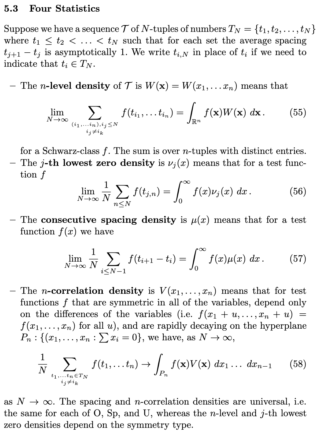
In addition to the pairwise distance statistics (for an individual L-function) and the lowest zero statistics (for a family), the research literature studies a number of other things you can measure. The amount of terminology around statistics for eigenvalues (or L-function zeros) can be (at least for me) a bit overwhelming. One thing I found helpful was this overview given by Conrey in his survey, explaining that there are four major statistics studied in all of these research papers. He also states a precise definition of each. We have talked only about the fourth one (in the case $n=2$, i.e. pair correlation) and the second one (for $j=1$, i.e. the lowest zero).

A spectral interpretation?

The title of Michael Rubinstein's thesis, written under Sarnak, is Evidence for a Spectral Interpretation of the Zeros of L-functions. Comments made in papers of Sarnak, Katz and others indicate that many experts seem to believe in the existence of a spectral interpretation, i.e. that the zeros of an L-function aren't just behaving statistically like eigenvalues, but they actually are eigenvalues of ... something.

If you watched the video by Taylor Dupuy posted recently, you saw a key source of the uncontainable excitement surrounding the dream of a spectral interpretation! This cohomological version is "Deninger's dream", a research program of Christopher Deninger going back, I think, all the way to the 90s. I'll include the same video again here for convenience, with the proof starting around 25:40, as well as the link to the preceding videos of his Riemann Hypothesis playlist.

The proposed proof strategy of Deninger relies not just on the existence of a spectral interpretation, but on an underlying cohomological formalism including in particular the Hodge star operator. In fact, Sarnak has been careful to point out that a spectral interpretation even if discovered may not in itself be enough to prove RH.

The difference between the function field and the number field realms is that in the first, there is a geometric explanation for why groups like the symplectic or unitary matrix groups appear. The short and simplified version is that a family in this setting is not just a sequence, but something parametrized by an algebraic variety, and this variety has a fundamental group (just like in topology, although defining the fundamental group for algebraic varieties is conceptually a bit different). In the number field world, there is no parametrizing variety for a family, since it's just a sequence indexed by the natural numbers, and hence there is no hope of defining a "fundamental group". However, these geometric notions are aspects of the dream of a future $\mathbb{F}_1$-geometry!

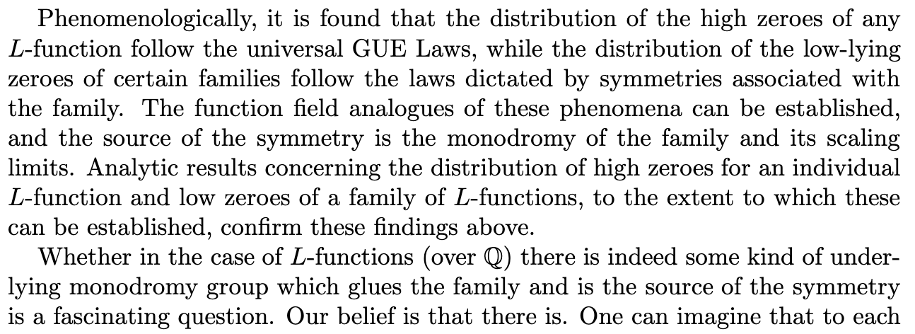
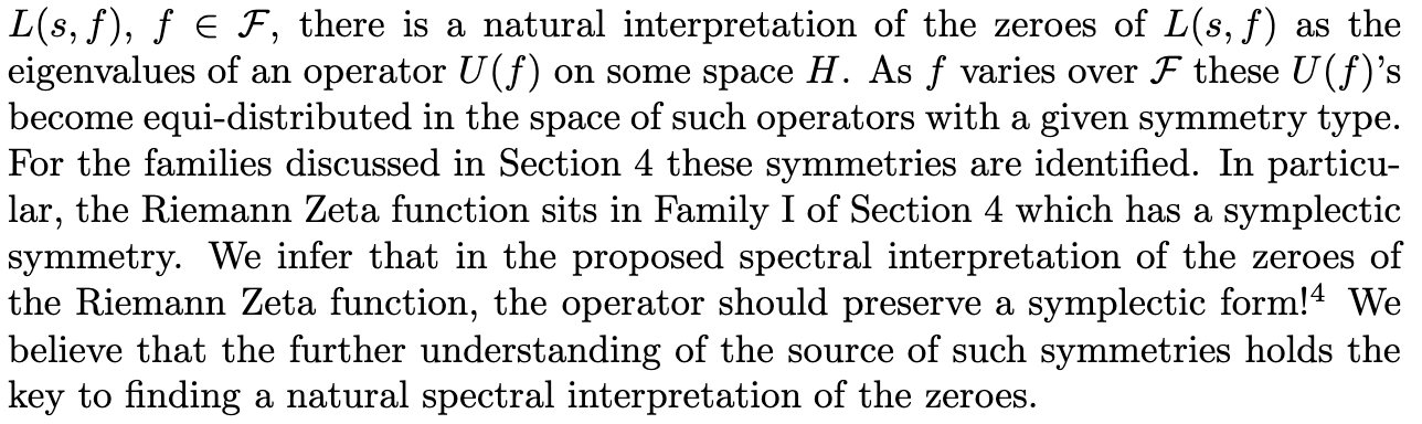
Here are the concluding paragraphs from Katz and Sarnak, to illustrate the uncertainty and hope expressed by experts. They believe in the existence of "some kind of monodromy group" for families in the number field realm, and they say one can imagine that there is a natural interpretation of the zeros of a given L-function as the eigenvalues of some operator.

References

The main references for this chapter were Conrey, Katz-Sarnak, and Sarnak-Shin-Templier. Before the paper of Sarnak, Shin and Templier, there were other attempts to capture the idea of a family, notably Sarnak's unpublished note from 2008 and Kowalski's Families of cusp forms, from 2013.

A general discussion on MathOverflow: What is the Katz-Sarnak philosophy?

A technical paper which was important historically because it treated "off-diagonal terms" is Iwaniec, Luo, and Sarnak: Low lying zeros of families of L-functions.

One of the great authors in the world of function fields is Douglas Ulmer. For connections to this chapter of the RH Saga, see Function fields and random matrices.

Advanced lecture notes by Philippe Michel covering many deeper aspects of L-function families, like the notion of subconvexity: Analytic number theory and families of automorphic L-functions.

A textbook covering some of what we've discussed is Miller and Takloo-Bighash: An invitation to modern number theory. I don't have a pdf link, but you'll find the TOC here. Also, two of the most interesting chapters are actually available online: Chapter 3 (introducing L-functions) and Chapter 15 (an excellent introduction to random matrix theory).

Finally, for the connections to nuclear physics: Nuclei, primes, and the random matrix connection, by Firk and Miller.