RH Saga Chapter 3: What does the Generalized Riemann Hypothesis really mean?

RH is a precise statement, and in one sense what it means is clear, but what it is connected with, what it implies, where it comes from, can be very unobvious.

Martin Huxley

Previously in the RH Saga, we introduced the "Big Five" problems motivating the idea of $\mathbb{F}_1$, and we reviewed the landscape of L-functions, together with some key ideas from the Langlands program. Today, we shall focus on the most famous of the Big Five, the Generalized Riemann Hypothesis.

Note: If you subscribe and read this as an email, the LaTeX may not render properly, and the interactive Sage code is completely invisible! Click the link above to read everything in the browser instead.

I want to explain (to the best of my limited ability!) what the Generalized Riemann Hypothesis really means. My attempt to do so will consist of three increasingly abstract levels of explanation, where each one (but most of all the last!) provides some clues to what one should look for when exploring ideas that could lead to a good theory of $\mathbb{F}_1$.

The first explanation is simply the visual, almost visceral, experience of seeing the zeroes of different L-functions bring forth different harmonies in the "music of the primes". Seeing these "prime waves" arising purely from the zeroes of an L-function, at least it should seem plausible that having strong restrictions on the location of the zeroes can give you deep insight into the nature of these different families of prime numbers.

The second explanation is the classical and rigorous discussion of generalized prime-counting functions. Just like the Riemann zeta function is connected to the classical prime-counting function $\pi(x)$ and its close relatives $\vartheta(x)$ and $\psi(x)$ (the first and second Chebyshev functions), every L-function has its own prime-counting function (or functions), and the GRH can be understood as giving precise bounds on the error term in asymptotic formulas for these functions.

Finally, in the third explanation I want to highlight three deeper themes intimately intertwined with the true meaning of GRH. In my view, the acid test for any proposed theory of $\mathbb{F}_1$ should be that it offers some genuinely new insight on at least one of these themes.

Music of the primes

The Generalized Riemann Hypothesis says that for every L-function $L(s)$, all zeroes in the critical strip actually lie on the critical line. That's the statement, and in some basic and tautological sense, it is also the true meaning of GRH. But how should we understand the deeper essence and significance of this problem, possibly the greatest unsolved problem of all time?

In the RH Saga Episode 3 video on YouTube, I tried to convey the connection between the zeroes of an L-function and the prime numbers, where each L-function appears to contribute its own theme or voice to the great "music of the primes" symphony. Here's that video in case you want to watch or rewatch it.

Recall that $L_A$ is one of the functions we now refer to as quadratic Dirichlet L-functions (with the notation $L_{-4}(s)$), and that $L_K$ is an example of a Dedekind zeta function, constructed from the Gaussian integers. In fact, it is a very simple example, since it is just the product of $L_A$ with the Riemann zeta function.

If you want to play around with the examples from the video, or (even better!) explore other L-functions too, like $L_D$ for any fundamental discriminant $D$, here is some Sage code for that.

First, in the widget below you can see the Dirichlet coefficients $a_1, a_2, a_3, \ldots$ for any of the above L-functions. Note that if you want to study $L_D$, you have to choose your own value of $D$ on line 9 of the code.

Alternatively, you can get the same Dirichlet coefficients as a simple list, so that you can use them as input for further computations.

Here is code for listing the spectrum, as a starting point for all kinds of further experiments. Choose LP, LE, LA, LK or LD on line 18 to see the spectrum of your favourite L-function.

And here is for plotting the zeroes, with an option to include the trivial ones.

Finally, here are the prime waves. Try to recreate all of the waves seen in the video, like the "heartbeat of love" for the prime $17$! For $L_K$, we saw spikes at $5$, $9$, $13$ and $17$. Does this regular pattern continue? Will there be spikes at $21$, $25$, $29$ and so on?

Exercises

At this point you can begin to explore the prime waves for our new friends, the Dirichlet L-functions $L_D$. Here are a few exercises to get going.

Exercise: In the video (timestamp 19:47), the question of patterns in the prime waves for $L_{-4}$ was left open. What is the pattern? What is the rule for where these spikes appear?

Exercise: The L-functions with $D = 8$ and $D=-8$ are special in that they share the same conductor (which is $\vert D \vert$, i.e. $8$). If you plot the prime waves for these two L-functions, what are the similarities? What are the differences?

Exercise: Explore the spectrum of $L_D$ for various values of $D$, and look specifically at the smallest element, i.e. the "lowest zero". How large can it be? How small can it be? Do you think there is a smallest or a largest possible value as we vary $D$ over all fundamental discriminants? Could you find a formula or algorithm that lets you compute this lowest zero, exactly or approximately, in terms of the discriminant $D$?

Generalized prime-counting functions

The classical Prime Number Theorem (PNT) gives an asymptotic formula for the size of a prime-counting function. The Riemann Hypothesis (RH) refines the PNT by giving precise information about the error in the asymptotic formula. Roughly speaking, the error will be of order $x^{\beta}$, where $\beta$ is the real part of the most mischievous of all Riemann zeta zeroes, i.e. the zero furthest away from the critical line. So if you can prove that all zeroes have real part at most $0.7$, you get an error term of order $x ^{0.7}$. If RH is true and all zeroes are on the line $\Re(s) = \frac{1}{2}$, the error will be of order $\sqrt{x}$.

Let's make this more precise. There are many equivalent ways of formulating both PNT and RH, and I want to review some of these variants. As always in the RH Saga, we emphasize statements and questions that can later be generalized to all L-functions.

Four counting functions for Riemann zeta

In order to construct a counting function to express the classical PNT and RH, you have to first decide whether to count primes ($2, 3, 5, 7, 11, 13, \ldots$) or prime powers ($2, 3, 4, 5, 7, 8, 9, 11, \ldots$). Second, you have to choose a weight for each prime or prime power, i.e. you have to decide how much a given element should contribute to your count. All in all, there are four different combinations that turn up naturally when you study the Riemann zeta function, and any one of these four can be used to express the statements of PNT and RH.

(1) The obvious choice of weight is of course $w=1$, and counting primes with this weight gives you the classical prime-counting function

\[ \pi(x) = \sum_{p \leq x} 1 \]

(2) Counting the prime powers with weight $w(p^k) = \frac{1}{k}$ gives a function used in Riemann's original paper.

\[ \Pi(x) = \sum_{p^k \leq x} \frac{1}{k} \]

(3) You can count primes with weight $w(p) = \log(p)$. This counting function is called the first Chebyshev function.

\[ \vartheta(x) = \sum_{p \leq x} \log(p) = \log \prod_{p \leq x} p \]

(4) Finally, you can count prime powers with weight $w(p^k) = \log(p)$. This gives the second Chebyshev function.

\[ \psi(x) = \sum_{p^k \leq x} \log(p) = \log \mathrm{LCM}(1, 2, 3, \ldots, n) \ \ \textrm{(LCM of all integers up to $x$)} \]

Note that every time you see a $\log$ in analytic number theory, it is the natural logarithm.

Variants: Each of the above functions is a step function that jumps at certain integer values. We can modify any step function so that the value at the jump point is redefined as the average of the value before and the value after the point. These modified functions are denoted by a subscript $0$. So for example, $\pi_0(11)$ is $4.5$ instead of $5$, since we now count the primes $2$, $3$, $5$, $7$, and "half" of $11$. These variants $\pi_0$, $\Pi_0$, $\vartheta_0$ and $\psi_0$ are often used not because it matters for the statements of PNT and RH, but because they are better behaved in relation to so-called explicit formulas. An explicit formula in analytic number theory is roughly speaking an identity relating a sum over primes (or prime powers) to a sum over zeta zeroes. We will come back to such formulas many times, in increasing level of detail.

Relations between prime counting functions and Riemann zeta

All of the four functions are related to each other through various transformation formulas, so that (with a little bit of work) you can transfer a statement about one of the functions to one about any other. Just to give one example of such a relation, Riemann's prime-power counting function can be expressed in terms of the second Chebyshev function like this:

\[ \Pi(x) = \frac{\psi(x)}{\log x} + \int_{2}^{x} \frac{\psi(t)}{t (\log t) ^2}dt \]

Also, all of the functions can be related to the Riemann zeta function. Again, just to give an example, we have the relation

\[ \log \zeta(s) = s \int_{0}^{\infty} \frac{\Pi(x)}{x ^{s+1}} dx \]

For another example of this sort, we have the explicit formula

\[ \psi_0(x) = x - \log(2 \pi) - \sum_{\rho} \frac{x^{\rho}}{\rho} \]

where the last sum is taken over all zeroes of $\zeta(s)$, including the trivial ones. \

It is a good exercise to work through these various relations (with proofs) for yourself. You can find much of what you need on Wikipedia (check Prime-counting function and Chebyshev function to get started), but you can also consult any standard text on basic analytic number theory, such as Montgomery and Vaughan: Multiplicative number theory I: Classical theory.

Statement of PNT

Recall the notation $f(x) \sim g(x)$, which simply means that $\frac{f(x)}{g(x)} \to 1$ as $x \to \infty$.

The Prime Number Theorem (proved independently in 1896 by Hadamard and by de la Vallée Poussin), says that

$\pi(x) \sim \frac{x}{\log x}$

In this statement, we could have replaced $\frac{x}{\log x}$ by any function with the same asymptotic growth rate, such as $\textrm{li}(x)$ or a certain function called the Riemann $R$ function. The definitions of these functions are

\[ \textrm{li}(x) = \int_{0}^{x} \frac{1}{\log t} dt \]

and

\[ R(x) = 1 + \sum_{k=1}^{\infty} \frac{(\log x) ^k}{k \cdot k! \cdot \zeta(k+1)} \]

So this is the classical prime number theorem, that $\pi(x)$ grows like $\frac{x}{\log x}$. Equivalent formulations would be that $\Pi(x)$ grows like $\frac{x}{\log x}$, or that one of the Chebyshev functions grows like $x$.

Statement of RH

Recall the "big-O" notation $f(x) = O (g(x))$, which means there is some constant $C$ such that $\vert f(x) \vert \leq C \cdot g(x)$. Intuitively, the growth rate of $f$ is not higher than the growth rate of $g$.

Now we can state the Riemann hypothesis! For this purpose, the expression $\frac{x}{\log x}$ is not precise enough; instead we must use $\textrm{li}(x)$ (and $R(x)$ would also work). The Riemann Hypothesis states that for every $\varepsilon>0$, we have

\[ \pi(x) - \textrm{li}(x) = O(x^{\frac{1}{2} + \varepsilon} ) \]

Intuitively, the error in the asymptotic formula does not grow faster that $x$ raised to the power "$\frac{1}{2}$ plus an infinitesimally small quantity". To make that last sentence into a precise mathematical statement, one can also formulate RH as

\[ \pi(x) - \textrm{li}(x) = O(x^{\frac{1}{2}} \log(x) ) \]

This looks like a strictly sharper statement, since $\frac{\log(x)}{x ^{\varepsilon}} \to 0$ for any $\varepsilon >0$, but is in fact equivalent.

We could also state the Riemann Hypothesis using any of the other three prime-counting functions. For example, in terms of the second Chebyshev function, RH says that

\[ \psi(x) - x = O( x^{\frac{1}{2} +\varepsilon}) \]

In this case, we can also give a seemingly sharper but equivalent version:

\[ \psi(x) - x = O( \sqrt{x} (\log x) ^2) \]

We haven't really touched on how to prove these prime-counting error bounds from the original RH statement (that all zeroes are on the line). But the idea is to use explicit formulas. For example, using the Riemann $R$ function, we have the relation

\[ \pi_0(x) = R(x) - \sum R(x^{\rho}) \]

where the sum is taken over all zeroes $\rho$ of $\zeta(s)$.

Explicit and Deep RH

Even though we have now formulated RH in a satisfactory way, there are two natural ways in which one might try to make the statement even more precise.

First, we could ask about the constant $C$ that is implicit (and unspecified) in the big-O notation. Can we find an explicit value for this constant? As mentioned before in a previous post, one can in fact use

\[ C = \frac{1}{8 \pi} \]

More precisely, this explicit version of RH says for any $x > 2657$, we have the inequality

\[ \vert \pi(x) - \textrm{li}(x) \vert < \frac{\sqrt{x} \log x}{8 \pi } \]

In a second direction, one could ask if the error bounds above can be improved further. If we focus on the error bound $O(\sqrt{x} (\log x)^2 )$ for the second Chebyshev function, the Deep Riemann Hypothesis says that this error bound is in fact

\[ o(\sqrt{x} \log(x)) \]

Here we use "little-o" notation, meaning that the error divided by $\sqrt{x} \log(x)$ goes to zero as $x\to \infty$. So this is stronger than the previous bound, both in the factor $\log x$ removed, and in that we changed from "big-O" to the stronger "little-o" type of bound.

Finally, the statement of GRH

After all of that background for the Riemann zeta function, we arrive at the statement of GRH!

Every L-function $L(s)$ has its own version of the second Chebyshev function, $\psi(x)$. For this general $L(s)$, the analogue of the Prime Number Theorem can be stated as

\[ \psi(x) \sim mx \]

where $m$ is the order of the pole of $L(s)$ at $s=1$. You may recall that the Riemann zeta function has a pole (a "vertical asymptote") of order one at $s=1$ (so $m=1$ in this case), while the graphs of $L_D(s)$ from the previous chapter showed nice and bounded behaviour around $s=1$, so no pole, and $m=0$ for these L-functions.

The Generalized Riemann Hypothesis says that for every $\varepsilon > 0$, we have

\[ \psi(x) - mx = O(x ^{\frac{1}{2}+\varepsilon}) \]

This is the "prime-counting" version of GRH, and all that remains now is to define what $\psi(x)$ is. One explanation is that we define $\psi(x)$ by counting prime powers like before, but instead of counting $p^k$ with weight $w = \log p$, we use the weight $w = b_{p ^k}$, where this last number is defined by writing the log derivative of $L(s)$ as a Dirichlet series, like this:

\[ - \frac{L'(s)}{L(s)} = \sum_{n=1}^{\infty} \frac{b_n}{n ^s} \]

In fact, the coefficients $b_n$ of the log derivative happen to be $0$ unless $n$ is a prime power. So in other words, if you write out the (negative of) the log derivative of $L(s)$, then each coefficient in this Dirichlet series is used as a weight in our new and generalized prime-counting function.

One final remark: If you already know about the Satake parameters $\alpha_1, \alpha_2, \ldots, \alpha_d$ at a prime $p$, then you can compute the weight $w$ more explicitly. The formula is

\[ w = (\log p) \cdot \sum_{j=1} ^d \alpha_j ^k \]

If you don't know what these numbers are, the brief explanation is that they are the reciprocal roots of the polynomial appearing in the Euler factor at $p$. But we will learn about them in the next chapter of the RH Saga!

One could of course ask if the GRH (just like RH) can be refined to seemingly sharper versions, explicit versions, or "deep" versions. But all of this is a story for another day.

To summarize this section, every L-function has it's own prime-counting function analogous to the second Chebyshev function, but with the weight of $p^k$ defined in terms of the Euler factor at the prime $p$. And from this point of view, the true meaning of GRH is the best possible error bound on the growth of this prime-counting function.

Complexity, Ramification, Positivity

These are three of the deepest concepts you will ever encounter in number theory. Each of them captures one important aspect of GRH.

Complexity

A few years after Enrico Bombieri wrote the official Clay Millennium Problem description for the Riemann Hypothesis, Peter Sarnak wrote another complementary description of the same problem. They are quite short, and obviously well worth reading in their entirety. Among the countless consequences that would follow from GRH, Sarnak chose to highlight four, as you can see below.

Note that he also says that for problems B, C and D we can get pretty far without knowing GRH, using alternative tools or weaker but unconditional substitutes of GRH. But for Problem A, no such progress is on the horizon with the tools we currently have! This Problem A says that there is a certain constant $C$ such that if the coefficients $a_1, a_2, a_3, \ldots$ of two elliptic curve L-functions agree for the first $C \log(N_1 N_2)^2$ coefficients, then the two L-functions must be the same! Here $N_1$ and $N_2$ are the conductors of the two L-functions.

So intuitively, the GRH implies that an L-function is determined by its first $P(\log(N))$ coefficients, where $P$ is some polynomial. The crucial point here is that the information content of an L-function (or its Kolmogorov complexity) is some power of $\log(N)$ as opposed to some power of $N$, an exponential improvement in the complexity bound.

For the L-function (in this case often called the zeta function) of a function field (i.e. the second column of Weil's Rosetta Stone), there is a geometric theory that explains this complexity phenomenon. The function field can be interpreted as a curve over a finite field, and this curve has an invariant $g$ called the genus (essentially the Euler characteristic) which is analogous to $\log(N)$. It follows from the Weil Conjectures that there is a set of $2g$ algebraic numbers (known as the Weil numbers) such that all of the zeta function coefficients can be computed from them in terms of very simple symmetric polynomials.

Going back to the number field world, one could dream (perhaps naively) that there is an integer invariant $G$ (the "$\mathbb{F}_1$-genus"?), roughly the size of $\log(N)$, such that every L-function comes with a list of $G$ numbers from which all coefficients can be computed. But nothing of this sort is known.

Ramification

Returning to the recent Harvard CMSA talk of Sarnak, you will find the following quote from around 19:57 to 21:00 in the video.

And then there's the discriminant. This is all about ramification/conductor. That's what the Riemann Hypothesis controls - it controls ramification in a very deep way. That's where the power of its applications come. So the discriminant is the places (the primes) at which the number field is ramified - the ramification is built into the discriminant through an integer and that appears in the functional equation.

So the functional equation now has this conductor, or complexity, and the most important thing is that the number of zeros that are locally... So if you go high up, you will have more and more zeros, but look low down. The number of zeros that a Dedekind zeta function will have will be $\log(D)$ over $2 \pi$. Logarithm! I urge you to note: Logarithm! That's going to allow me to transcend complexity classes. Log of the conductor is the number of zeros, and the number of zeros (if you are polynomial) would be related to the degree, clearly the complexity. So the log of the conductor is like the degree.

The quote is from a context where he introduces the GRH for general L-functions, using a Dedekind zeta function as a representative example. So you see (again!) the emphasis on $\log(N)$ as a complexity measure, with an implicit reference to the function field world, where the L-function really is a polynomial. In the basic case of curves, this polynomial has degree $2g$, and the zeroes come in $g$ complex-conjugate pairs.

I will be honest and say that this statement of Sarnak, that GRH "controls ramification in a very deep way", is not a statement I understand fully. But it gives a very significant clue in that if we are serious about trying to construct an $\mathbb{F}_1$-geometry relevant for the Riemann Hypothesis, then the geometry must in some way explain or encompass phenomena related to ramification. I can show you at least some fragments of these phenomena here and now, and hopefully we can come back to ramification many times in future lectures, adding more pieces of understanding to the puzzle.

One of the most important invariants of an L-function is its conductor $N$. If you look at a plot of the spectrum, like we did above, you may notice that the zeroes slowly become more and more dense as we move up the critical line. Here is a plot generated by the Sage code above, for the Dirichlet L-function with $D=5$.

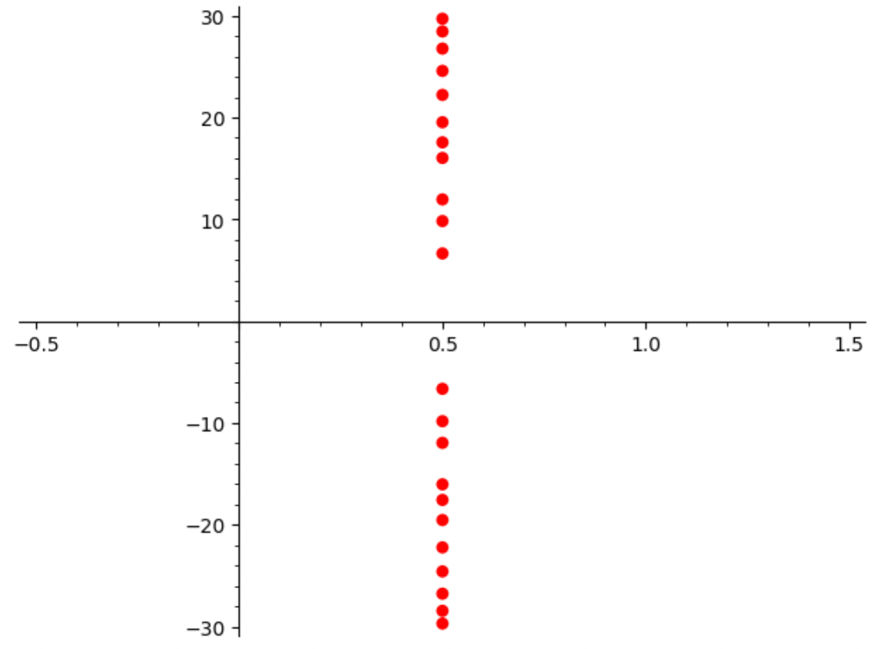
Let's count the zeroes above in the case of a Dirichlet L-function, let's say from imaginary part $0$ to $T$ (the picture shows $T=30$). You can count them yourself in the picture above to see that the number is $11$. The asymptotic formula for the number of zeroes (for this specific L-function) is

\[ \frac{T}{2\pi} \log (\frac{5 T}{2 \pi e}) \]

and plugging in $T=30$ gives $10.4$. Not bad!

The general asymptotic formula for the number of zeroes up to height $T$ in the critical strip is

\[ \frac{T}{2\pi} \cdot \log \frac{N T ^d}{(2 \pi e) ^d} \]

This formula is valid for any L-function of conductor $N$ and degree $d$. So for the L-function $L_E$ in the video, you can now use $N=14$ and $d=2$ and check for yourself how good (or bad) this formula is compared to the actual count of zeroes up to various heights.

Anyway, the point I wanted to illustrate is that ramification information (packaged in the conductor $N$) governs the density of the zeroes on the critical line.

One should compare this situation to L-functions from the realm of function fields. For these functions, the zeroes in the critical strip do not grow denser as we move up the line! Instead, there is a finite set of zeroes which just repeat forever. In the basic case of a curve over the finite field $\mathbb{F}_q$ (with $q$ elements), the number of zeroes up to height $T$ is approximately

\[ \frac{T}{2 \pi} \cdot 2g \log q \]

Here we are at the heart of $\mathbb{F}_1$ mystery! The two formulas are analogous. But the number $q$ does not have a precise analogue in the number field world (naively setting it to $1$ would make no sense in this specific context, as we would get $\log(0)$). So you can sort of see that $2g \log q$ appears where we for number fields have $\log(N)$. In other words, the conductor $N$ is analogous to the factor $q^{2g}$. But the factor $(\frac{T}{2 \pi e})^d$ does not appear at all in the function field world! Still, part of the dream is that the geometric language for ramification theory in the world of function fields will have some counterpart in the world of number fields.

One of the problems with some existing proposals for $\mathbb{F}_1$-geometry is that they only cover L-functions which come from toric varieties. Without going into technical details, a quick explanation is that toric varieties are varieties with conductor $N=1$, meaning that there is no ramification at all. This is a major (I would say fatal) drawback if the purpose of the $\mathbb{F}_1$-geometry is to say something about the Riemann Hypothesis. Ramification must be part of the theory.

I can mention one concrete open research problem relating to conductors. One could hope that a good future theory of $\mathbb{F}_1$ could say something about this problem. One of the best short introductions to L-functions is Henri Cohen's Computing L-functions: A survey, from 2015. Here on page 7 (page 704 in the published version) you see (for various choices of Gamma factor) some small values of $N$ that can occur for an L-function. These lists look completely chaotic! In the first two cases, we're talking about our friends the Dirichlet L-functions $L_D$, with positive and negative $D$ respectively. In these cases the values correspond to fundamental discriminants, and we understand which values of $N$ appear. But in all other cases we have no idea! For example, which numbers $N$ appear as the conductor of an elliptic curve over $\mathbb{Q}$?? The list (which you can explore further in the LMFDB) begins with $11, 14, 15, 17, 19, 20, 21, 24, 26, 27, \ldots$.

Positivity

The third deep theme I want to introduce today is positivity. One could say that GRH expresses the positivity of certain invariants. If you recall the Keiper-Li coefficients of an L-function from Episode 6, you know that the GRH is equivalent to all these numbers being positive.

In fact, in Sarnak's talk from 2018, he says that all approaches to GRH rely on positivity in one form or another. Check the slides here, where on page 3 he says "What is known about GRH? All methods are based on positivity."

Positivity comes in many guises, and we certainly don't have the final theory that could explain something like the positivity of the Keiper-Li coefficients. The simplest setting is the elementary trigonometric inequality

\[ (1+\cos(\theta))^2 \geq 0 \]

which is a key input to the proof of the Prime Number Theorem. This proof is carefully explained in Romik's notes, around page 70.

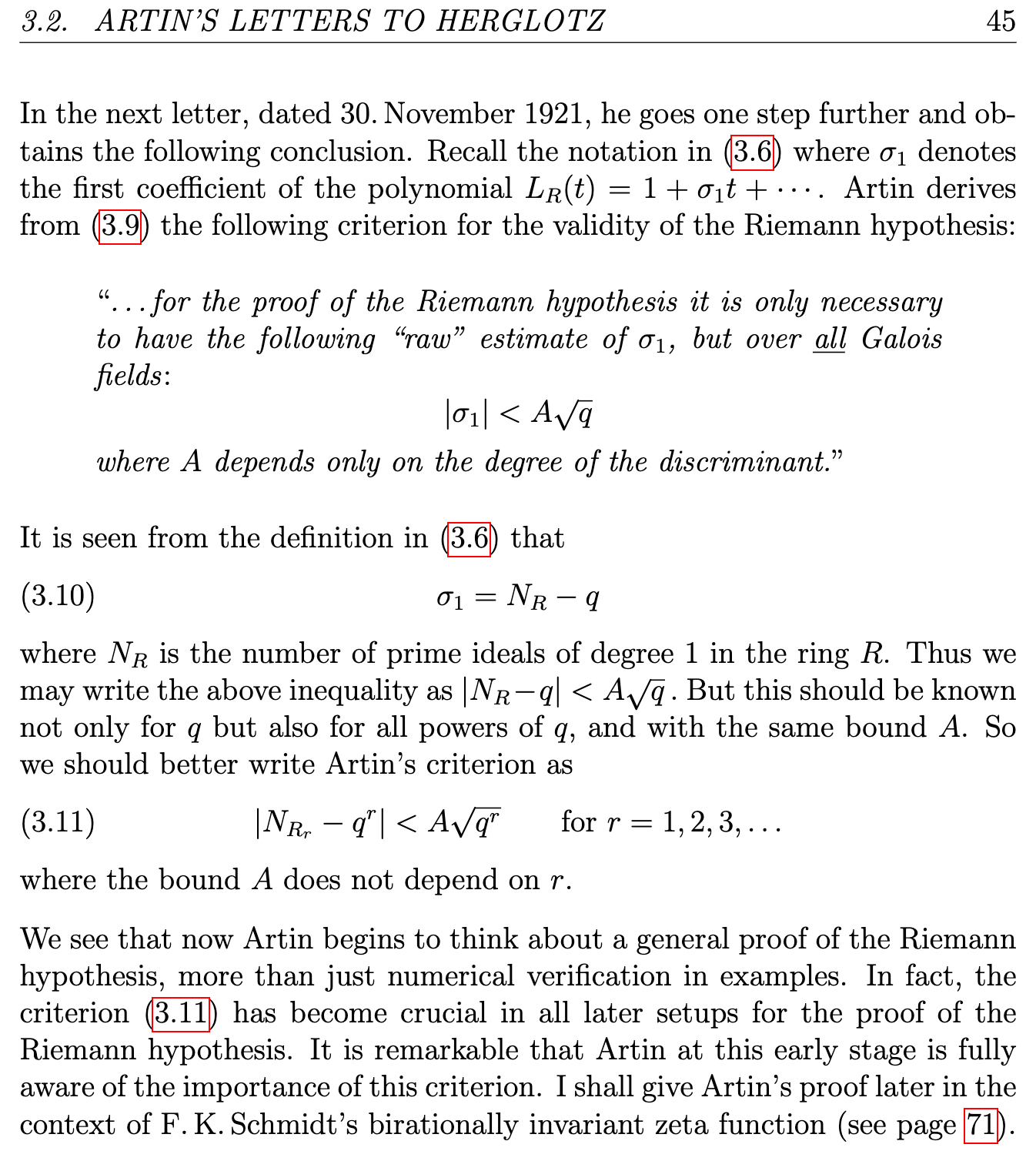
Just to give one connection to the world of function fields, I will show you part of page 45 in Roquette's remarkable historical survey of RH for function fields. In this context we have a criterion implying RH that goes all the way back to Artin's thesis. The page in question speaks for itself. But note the key point, that the criterion relies completely on being able to extend the finite field $\mathbb{F}_q$ to larger and larger finite fields $\mathbb{F} _{q ^r}$. And this process (sometimes called "adjoining roots of unity", or "extending the field of constants") does not have a counterpart in the world of number fields, since we don't have a good definition of $\mathbb{F} _{1}$ or it's hypothetical extensions $\mathbb{F} _{1 ^r}$.

To summarize, the true meaning of GRH, from a deeper and more abstract point of view, is that it (1) governs the Kolmogorov complexity of an L-function, (2) controls ramification "in a very deep way", and (3) expresses some mysterious inequalities referred to as "positivity". A good future theory of $\mathbb{F}_1$ should connect to all of these ideas.

Explorations

To end this chapter, I will propose two exploratory projects for which you now have all the necessary tools. Any of these could be an excellent topic for the Essay competition!

Problem 1: Second Keiper-Li coefficient of $L_D$

In the case of Dirichlet L-functions, the first Keiper-Li coefficient is well understood, but the second is not! Below is some Sage code that computes the second Keiper-Li coefficients for any $L_D$.

Do these numbers grow with $D$ or are they more irregular? Can you find any rules, patterns, or formulas in these numbers? What kinds of ideas or structures could lead to a proof that these numbers are positive?

Problem 2: Gaussian primes

Consider the Gaussian integers seen in the Episode 3 video. Some of these integers are prime, meaning they cannot be factored unless one of the factors is a unit.

Prime elements in the Gaussian integers are grouped together in groups of four, so that within a group each element can be obtained from any other by multplication by some unit (equivalently, by a sequence of $90$-degree rotations around the origin). If we count these groups of primes instead of the prime elements themselves (technically, this corresponds to counting prime ideals), we get a counting function looking like this:

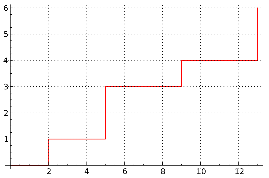
Gaussian prime counting graph, from Mazur and Stein

1) Find by hand all the small Gaussian primes, and check that they correspond precisely to the above step function. Can you find the general rule for when the step function jumps (and by how much)?

2) Can you find an expression for the step function in terms of the zeroes of $L_K$? Look for a formula analogous to the one above for $\pi(x)$.

3) Write some code to plot the Gaussian primes in the complex plane. Do you find any interesting patterns?

4) To keep going with the remarkable world of Gaussian primes, you can follow the amazing and highly readable paper by Harvard mathematician Oliver Knill, where he goes step by step into increasingly exotic territory, including primes in the realm of quaternions!