
RH Saga Chapter 6.1: Exponential invariants

Recall from last time that natural invariants of L-functions tend to fall within one of three different classes: Additive, exponential, and lambda-additive.
Today I want to walk through the exponential invariants, with some brief comments on each.
Root number
Any L-function has a root number $\varepsilon$, also called the sign, which is a complex number of absolute value one. It appears in the functional equation of the (completed) L-function; here in Axiom 2 from Farmer, Pitale, Ryan and Schmidt.
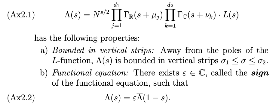
The history of the theory of root numbers is full of interesting and important chapters. For the degree-1 case of Dirichlet L-functions, the root number can be expressed in terms of the Gauss sum attached to a Dirichlet character, and it took Gauss several years to prove that for a quadratic Dirichlet character, the root number is always equal to $1$.
An important aspect of the theory is that the root number can be factorized into a product of local root numbers, one for each prime (including the "prime at infinity"). For example, in the case of an elliptic curve L-function we have
$\varepsilon = - \prod_p w_p$
where one should think of the minus sign as the "local root number at infinity", and the rules are that $w_{p} = 1$ whenever $p$ is a good prime, $w_p = -1$ when $p$ is split multiplicative, and $w_p = 1$ when $p$ is non-split multiplicative. For the remaining case where $p$ is additive, there is a number of subcases giving either $1$ or $-1$. Finally, for the primes $2$ and $3$ the theory is more complicated, and complete tables of different cases were published by Halberstadt in 1998.
Conductor
The conductor of an L-function is the positive integer $N$ appearing in the completed L-function as seen above. We have discussed the conductor on several occasions already, notably in Chapter 2. It can be written as a product
\[ \prod p^{f_p} \]
over all the bad primes, where $f_p$ is the conductor exponent at $p$.
Analytic conductor
The analytic conductor $A$ is a more refined measure of complexity of an L-function than the ordinary conductor. Here is the definition as formulated on the LMFDB Knowledge page. In other words, $\log(A)$ is the sum of $\log(N)$ and a term coming from the log derivative of the gamma factor, evaluated at $s=\frac{1}{2}$.
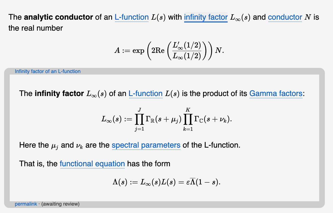
You may recall from the most recent talk of Sarnak (around slide 5) that he discusses a few variations on the definition of $A$, and the idea that $\log(A)$ measures the local density of the nontrivial zeros of the L-function near the central point on the critical line.
The special value at $m$
Fix a complex number $m$, which is all interesting cases will be either an integer or a half-integer. Evaluating the L-function at $m$ gives an invariant $L(m)$, which we call the special value at $m$. Note that some authors operate with restrictive conventions for what is meant be a "special" value, imposing some conditions on $m$, but for our purposes, it makes sense to be inclusive and allow any $m$.
The theory of special values is a massive story in itself, to which we shall return in upcoming chapters!
The leading term at $m$
Sometimes, the value at $m$ will be zero, and in this case, we can consider the Taylor series of the L-function at $s=m$, and define $L^{*}(m)$ to be the first non-vanishing Taylor coefficient. For example, at the central point of an elliptic curve L-function, this will be the $r$'th coefficient, where $r$ is the analytic rank.
The special value and the leading term (at some fixed $s$-value $m$) are both multiplicative invariants. A variation on these definitions is obtained by using the completed L-function instead.
Final remarks on higher Taylor coefficients
One could also study Taylor coefficients (and in the case of a pole at $m$ we should say Laurent coefficients) beyond the leading one. Such a coefficient is not in itself an exponential invariant in the sense defined here, but in some cases, it still carries deep arithmetic information.
Example: The Riemann zeta function has a pole at $s=1$ and the Laurent coefficients in this case are the Stieltjes constants.
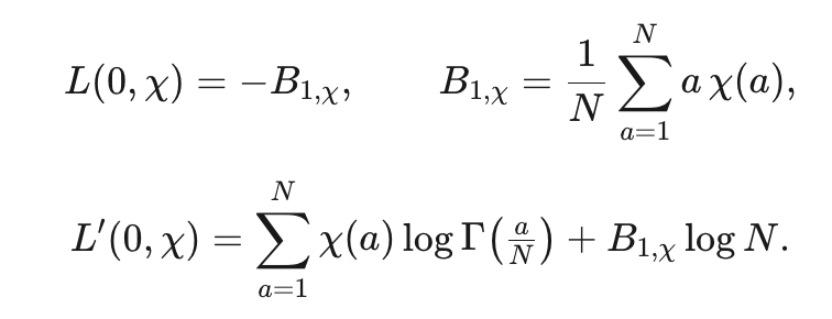
Another example: For a Dirichlet L-function (of conductor $N$), the derivative at $s=0$ is given by a finite sum of logs of fractional Gamma values! A generalized Bernoulli number also enters the formula, as follows:
Finally, as inspiration for $\mathbb{F}_1$, a 2017 Annals paper of Yun and Zhang studies Taylor coefficients at the central point for a class of L-functions in the function field world, and they show that all of these coefficients have a geometric interpretation, as intersection numbers on a moduli stack of shtukas. Any similar interpretation in the number field world would be a strong pointer to a possible $\mathbb{F} _1$-geometry!